
In the first post I described my experiments with the k-means algorithm, starting with my Clustering and Dimensionality Reduction course through Train in Data. While I usually play around with the examples they provide I became particularly interested in this area, creating a variety of alternative implementations and test scenarios. Eventually I needed to create a test framework covering timing, memory tracking, datasets, and initialization strategies to organize and track my work.
In the process of trying to optimize different algorithms I became convinced that the nested loops and independent calculations would be a natural fit for GPU acceleration, so I began investigating in that direction.
This post gets into what a GPU does differently, how PyTorch, one of the most common ways to program GPUs, maps onto that hardware, and why a specialized library called KeOps was ultimately the right tool for the job.
In addition I’ve created a short video where I experiment with the Manim library to visually walk through some of the concepts covered in this article. This may be a useful companion to the potentially dry text in this post.
tl;dr
GPUs are fast because they do simple things billions of times simultaneously. That works well for k-means. But PyTorch, the default for programming GPUs, uses lots of memory, which also makes it slow. KeOps uses far less memory, and ends up 10x faster as a result. You have to read on to learn why…
CPUs and GPUs are designed for different things
A modern CPU has a small number of powerful cores — typically somewhere between 8 and 32 on a high-end chip. Each core can handle complex, branchy logic: conditionals, function calls, memory accesses that depend on previous results. CPUs are optimized for latency, meaning they’re designed to finish any single task as fast as possible. They do this through mechanisms like deep instruction pipelines, large caches, and sophisticated branch prediction. The result is a chip that is extraordinarily good at handling one complicated thing after another.
A GPU is built around a very different tradeoff. A modern GPU has thousands of smaller cores, each considerably simpler than a CPU core. What they can do in parallel, though, is enormous. A GPU is optimized for throughput so it can perform a huge volume of similar independent operations. Individual cores are slower and less capable than CPU cores, but the sheer number of them working simultaneously compensates for that, many times over, for the right kind of work.
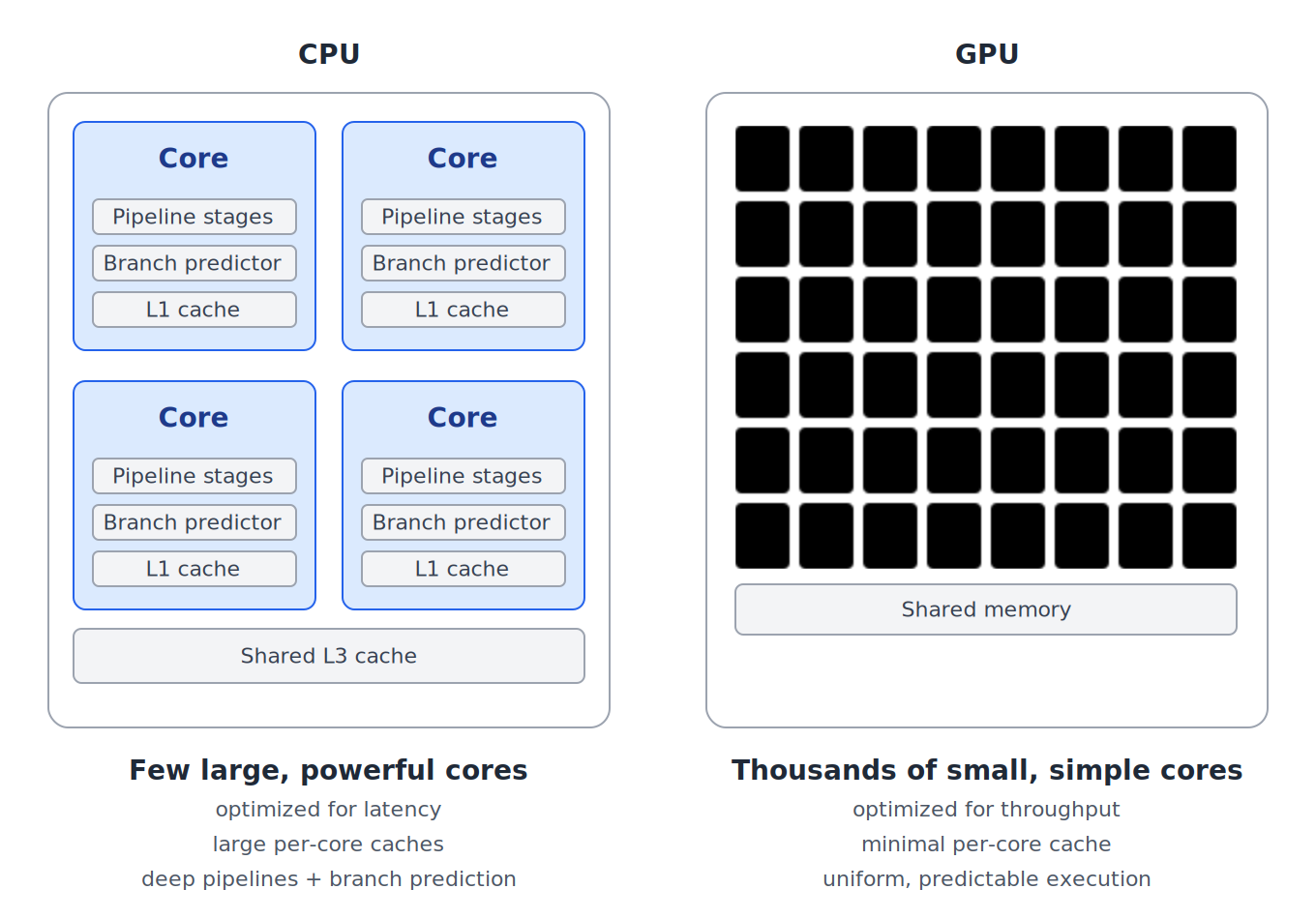
The right kind of work, in this context, means operations that are uniform and independent. If you have a million values and need to multiply each one by two, a GPU can hand one value to each of a million cores and finish the job nearly instantaneously. If you have a million operations that each depend on the result of the previous one, a GPU offers almost no advantage — the operations have to run in sequence regardless.
Why k-means fits this model
The assignment step in k-means is almost a textbook example of GPU-friendly work. For every data point, you need the distance to every centroid. Each of those distance calculations is independent: the distance from point A to centroid 1 has nothing to do with the distance from point B to centroid 2. There are no dependencies between calculations, no branching logic, and the operation is the same for every pair. With N points and K centroids, you have N times K independent calculations to perform, all identical in structure.
This is exactly what GPUs are built for. The question is how to express the computation in a way that actually lets the hardware work in parallel, rather than sending it one calculation at a time.
How PyTorch expresses parallel computation
PyTorch, the most widely used framework for GPU-accelerated numeric computing in Python, handles this through a concept called tensorization. Rather than writing a Python loop that computes one distance at a time, you express the entire computation as an operation on arrays — called tensors — and PyTorch dispatches that single operation to the GPU, which handles all the elements in parallel.
The trick for k-means is getting all the pairs (every point against every centroid) into a single operation. This is done through broadcasting. If you have N data points and K centroids in D dimensions, you can reshape the data tensor from shape (N, D) to (N, 1, D) and reshape the centroids from (K, D) to (1, K, D). The lone 1 in each shape tells PyTorch that this dimension should be expanded (broadcast) to match the other tensor. When you subtract them, PyTorch implicitly pairs every one of the N points with every one of the K centroids, producing a result of shape (N, K, D) — the difference between each point and each centroid, across all dimensions. Squaring and summing across the last dimension gives you an (N, K) matrix of distances, and taking the position of the minimum in each row gives you the cluster assignment for each point, all in a handful of lines with no Python looping required.
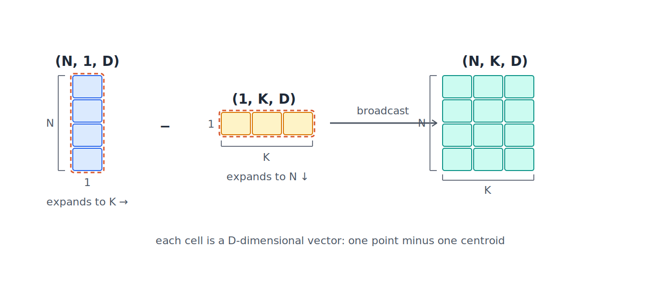
This is substantially faster than writing the equivalent loop in Python, which would send the CPU on a trip through N times K sequential operations while the GPU sat mostly idle. The tensorized version sends the whole job to the GPU at once.
Where PyTorch breaks down
There is a cost, and it shows up in memory. When PyTorch computes that (N, K, D) subtraction, it has to store the full result somewhere. On a GPU, that means GPU memory (VRAM). With 5 million points, 12 clusters, and 18 dimensions in 32-bit floating point, that intermediate result takes up roughly 4.3 gigabytes per iteration, and the benchmarks showed a delta of 5 GB of VRAM consumed by the tensor implementation on that dataset. PyTorch evaluates operations eagerly, producing a concrete result the moment you ask for one, so that tensor gets written to GPU memory at every iteration of the algorithm, for every value of K you sweep through.
On small datasets this doesn’t matter. On large ones it becomes a constraint. A 16 GB GPU is a reasonable mid-range research card, and a single K value sweep on a large dataset can consume the majority of that budget. If you push further by adding more K values, higher dimensional data, multiple restarts, you run the risk of running out of memory.
This is the problem KeOps was designed to solve.
KeOps: kernel fusion
KeOps, short for Kernel Operations, is a library that lets you express the same computation as PyTorch but avoids writing the intermediate result to memory at all.
The key concept is a LazyTensor. When you create a KeOps LazyTensor, you’re not asking it to compute anything yet. You’re describing a computation (a formula) that KeOps records but doesn’t evaluate. When you then ask for the result you actually need, such as the index of the nearest centroid for each point, KeOps generates and compiles a CUDA kernel that performs the entire computation in a single pass. For each point, it streams through all K centroids, computes distances one at a time, and tracks only the running minimum. The individual distance values exist momentarily in the GPU core’s registers and are immediately discarded. Nothing is written to GPU memory except the final answer: one cluster assignment per point.
The difference in memory scaling is significant. KeOps avoids writing the intermediate results to memory. In practice, at 500,000 points with 50 dimensions and K=12, the PyTorch approach allocates around 1.2 GB per iteration for that one intermediate tensor. The KeOps version uses well under 200 MB across the entire run.
Examples
| Dataset | sklearn | PyTorch | KeOps | PyTorch peak VRAM | KeOps peak VRAM |
| Wine K=3 | 0.007s | 0.021s | 0.040s | 0.009 GB | 0.009 GB |
| SUSY K=12 | 37s | 32s | 3.8s | 10.2 GB | 1.8 GB |
Table 1: Comparing implementations with Wine dataset (178 points, 13 dimensions, K=3) and SUSY dataset (5 million points, 18 dimensions, K=12) makes the tradeoffs concrete. This was run on Kaggle with GPU T4 x 2.
On the Wine dataset, sklearn is fastest. The GPU implementations all lose to the CPU because there is so little work to do that the overhead of dispatching to the GPU (sending the data structures) costs more than the computation itself. On SUSY the picture reverses sharply. KeOps is roughly ten times faster than sklearn and eight times faster than plain PyTorch tensor, while consuming about a fifth of the memory. The tensor implementation is barely faster than sklearn despite running on a GPU, because it requires large amounts of memory and spends considerable time reading and writing that memory.
There is a tradeoff. KeOps compiles its CUDA kernel the first time it encounters a new formula, and that compilation takes several seconds. Any benchmarks need to account for this: run each KeOps call twice and discard the first result. After the warmup, subsequent calls use the cached kernel. For a one-off analysis this warmup cost may be noticeable but not prohibitive. For production code that runs the same formula many times, it disappears quickly.
KeOps does not replace PyTorch. It handles a specific class of structured pairwise computations like distance matrices that PyTorch’s eager evaluation handles poorly at scale. For everything else, PyTorch remains the right tool.
One thing I tried was pushing the tensorization approach harder. The standard PyTorch implementation runs each random restart sequentially, with a Python loop around each one. If you batch all the restarts into a single tensor operation, stacking all the initial centroids into a three-dimensional array and running the distance computation across all of them simultaneously, you eliminate all of the Python loops and theoretically recover some throughput.
This turned out to be slower and more memory-intensive than KeOps at scale, not faster. The reason is the same memory problem in a different form. Batching all restarts simultaneously multiplies the memory pressure by the number of restarts. You’re not avoiding the intermediate tensor; you’re creating several of them at once. At large N the approach exhausted memory faster than the sequential version. The fundamental issue is that kernel fusion, not parallelism alone, is what actually solves the memory scaling problem. Trying to out-parallelize it with standard PyTorch tensors just runs into the same wall at higher speed.
When does GPU acceleration actually help?
The Wine and SUSY dataset numbers bracket the answer. At small N (data points), GPU overhead dominates and a well-optimized CPU implementation like sklearn wins. At 5 million points the GPU advantage is clear and the memory constraint becomes the real story — plain PyTorch tensor is fast enough in principle but its memory consumption makes it impractical for any serious sweep across K values on a system with limited memory. KeOps sidesteps that constraint entirely, which is why it remains fast even as N grows.
The other dimension that matters is D (dimensions). KeOps’s kernel fusion approach is particularly effective at moderate dimensionality. At very high D, data with a high number of dimensions such as raw image pixels or text embeddings, the register pressure increases and matrix-multiplication-based approaches like FAISS become more competitive.
For datasets with many points and moderate dimensionality, KeOps is worth the setup cost. For small datasets, sklearn is simpler and faster. For very high-dimensional data or multi-GPU scenarios, FAISS is worth considering.
While working on this I came across FAISS, a library developed by Meta AI Research that also addresses large-scale nearest-neighbor computation, which is what the k-means assignment step fundamentally is. FAISS takes a different architectural approach, using highly optimized matrix multiplication routines (specifically, the cuBLAS library on NVIDIA hardware) rather than kernel fusion. For datasets with very high dimensionality FAISS’s approach gives it an advantage, because matrix multiplication at high D is where cuBLAS is particularly well-optimized.
FAISS also supports multi-GPU scaling, which KeOps does not. At the scales tested in this notebook, the two libraries should be broadly comparable in runtime. For the datasets I was working with, KeOps was a natural fit; for applications involving very high-dimensional data or multi-GPU environments, FAISS is worth a serious look when I have time.
Coming Soon
So far I’ve covered the process of investigating k-means, creating a framework, and experimenting with KeOps to tune the GPU implementations. Up to this point in my work I had stuck with the ‘elbow calculation’ for determining the best value of K to use. I knew I should investigate the silhouette scoring technique, but put that off for a while. Eventually I reached a point where I wanted to ensure that I had good values of K to compare in my algorithms, and really flesh out the functionality of my framework, so I knew I had to implement silhouette scoring.
I’ll go into this algorithm and the various approaches I took to working with it in my next post.