
In the first post I described building a test framework for k-means clustering: timing, memory tracking, a range of datasets, and shared centroid initialization to make cross-implementation comparisons fair. In the second post I dug into what a GPU actually does differently from a CPU, how PyTorch expresses parallel computation through tensorization, and why KeOps (a library that compiles symbolic tensor computations as fused CUDA kernels) solved a memory scaling problem that plain PyTorch could not. The short version of that story: at small N, sklearn works well enough. But by the time you have five million points, KeOps is roughly ten times faster than sklearn and uses a fifth of the VRAM that a fully tensorized PyTorch implementation requires.
My work to this point was focused on algorithms for calculating k-means values. If you are familiar with this algorithm or read through the previous posts you might remember a key factor: The best value for K (where K is the number of clusters to group the data into) is often not known ahead of time.
The K Selection Problem
K-means requires you to choose K in advance. Sometimes the right K is obvious from domain knowledge. If you’re grouping data by months in a year, you would pick 12. More often, you don’t know, and you have to search. The standard approach is to repeatedly run the algorithm across a range of K values and look at how inertia, the sum of squared distances from each point to its assigned centroid, changes as K increases. The need to run k-means multiple times is one reason for finding quick, memory efficient algorithms.
The problem is that inertia always decreases as K goes up. At the extreme, if K equals the number of data points, every point is its own cluster and inertia is zero, which is obviously useless. What you’re looking for is an “elbow” in the inertia curve, a point where adding more clusters stops buying you much improvement. In practice the elbow is often subtle or ambiguous. Inertia is also sensitive to the scale of the data and the number of dimensions, which makes it hard to compare across datasets or to use as an absolute measure of quality.
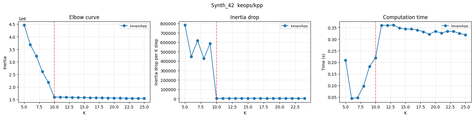
figure 1: This is the output from my k-means analysis. The first chart shows the inertia, with a clearly distinguishable elbow at 10. But also note that inertia continues to shrink past the elbow.
Silhouette Scoring
The silhouette score is a more informative way to evaluate clustering quality. It measures, for each data point, how well that point fits its assigned cluster compared to the next closest cluster. The result is a number between -1 and 1. A score near 1 means the point is well inside its cluster and far from its nearest neighbor cluster. A score near 0 means the point sits roughly on the boundary between two clusters. A negative score means the point may have been assigned to the wrong cluster entirely.
Computing the silhouette score for a point involves two quantities. The first is the average distance from that point to every other point in its own cluster. The second is the average distance to every point in the nearest neighboring cluster. The silhouette score is then the difference between those two, divided by whichever is larger. You can compute this per point, and then average across all points to get a single score for a given clustering.
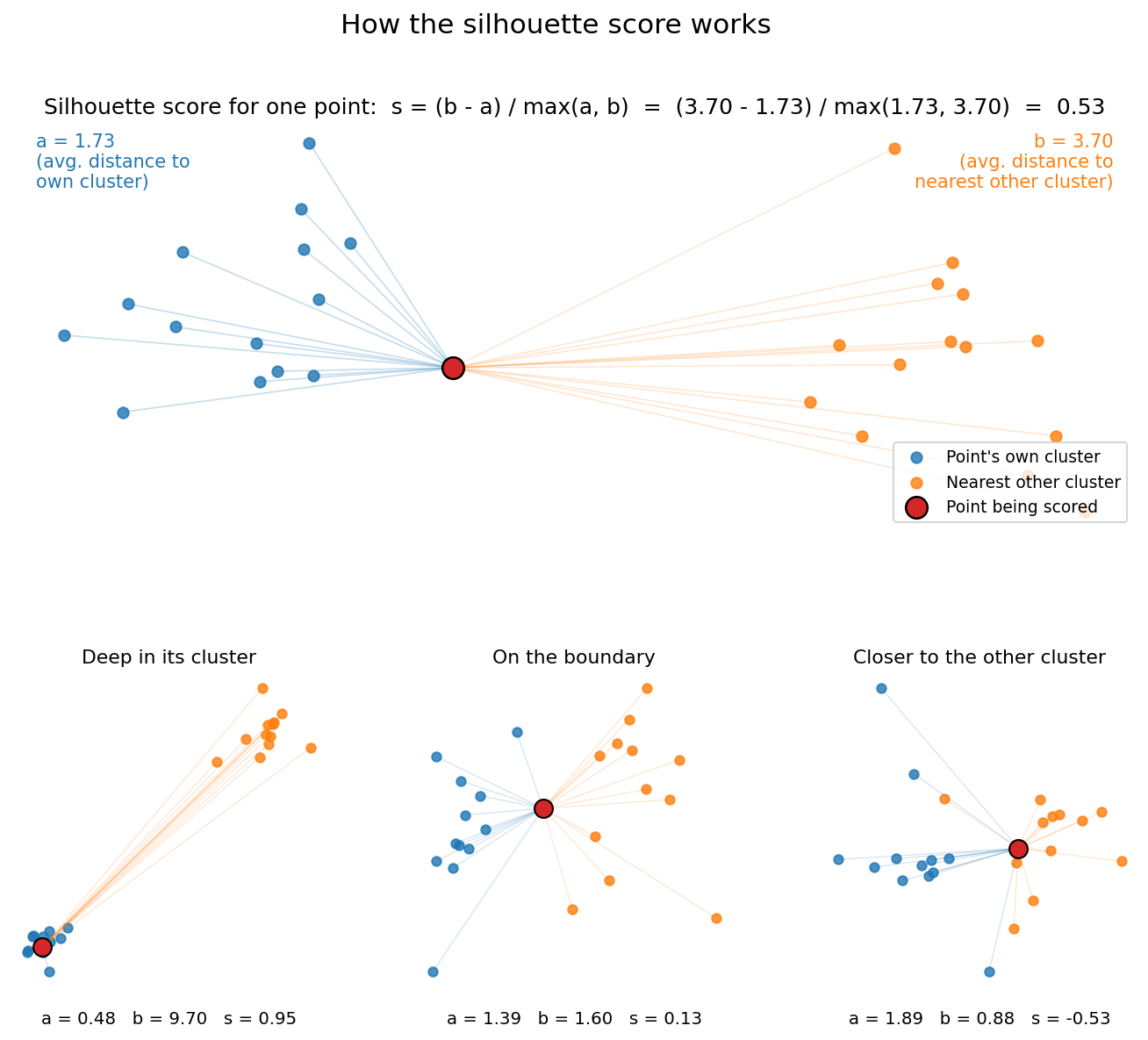
figure 2: The silhouette score in action
The practical value is that silhouette gives you something meaningful to compare across different values of K. Rather than watching inertia steadily decrease and trying to spot an elbow, you can look for the K that maximizes the silhouette score. A good clustering, one where points are genuinely closer to their own cluster members than to any other cluster, will produce a high average score. A K that splits a natural cluster or merges two distinct ones will produce a noticeably lower one.
The Scaling Problem, Again
The silhouette calculation looked similar to the k-means calculation. For each of the N points, computing the average distance to every point in the same cluster requires visiting every other point in that cluster. Computing the distance to the nearest neighboring cluster requires visiting every point in every other cluster. The total number of distance calculations is on the order of N squared.
For small datasets this is fine. For the SUSY dataset with five million points, it is not remotely feasible. You would need to compute and store something like 25 trillion distance values. Even with a GPU, the memory (VRAM) requirement would be impossible to meet.
This is the same challenge I encountered with k-means so I approached it in a similar fashion. I had the framework. I’d found some success with the GPU implementation of the k-means algorithm. I decided to experiment and see how various silhouette scoring algorithms worked with GPUs
Three Implementations
The first implementation used standard PyTorch to compute the full N by N distance matrix explicitly. This is exact and relatively straightforward to implement, but the memory cost is O(N squared). On a 16 GB GPU it held up further than I expected, running cleanly through 60,000 points before failing at 65,000. It serves the same role as the sklearn baseline did for k-means: a control implementation against which I could verify the others.
The second implementation used KeOps. The structure of the silhouette computation is pairwise distances between all points, then a reduction. This is exactly the kind of structured operation that KeOps is designed to handle. The LazyTensor approach avoids materializing the full distance matrix, keeping memory at O(N times K) rather than O(N squared). At large N this is not a minor improvement; it’s the difference between running and crashing.
The third implementation was an approximation, Simplified Silhouette Score. Rather than computing distances from each point to every other point in its cluster, I used the centroid of each cluster as a stand-in. This reduced the problem to N times K distance calculations, the same structure as the k-means assignment step, and is extremely fast. The tradeoff is accuracy. Distance to a centroid is not the same thing as average distance to every other point in the cluster, and the two diverge more as clusters become elongated or non-convex. The approximation holds up best on clusters that are roughly spherical, a well known limitation of the method.
Even under close to ideal conditions, in every test I ran, from a few hundred points up through a hundred thousand, my centroid version inflated the silhouette score by a fairly consistent 0.11 to 0.13. It’s a fast, useful estimate with low memory requirements, but the number it produces should be read as an approximation.
Verification of the algorithms followed the same pattern as k-means. I ran all three implementations on small datasets where the PyTorch version could produce exact results, confirmed that the KeOps scores matched to within floating point tolerance, and noted where the centroid approximation diverged. The KeOps implementation passed consistently.
What the Benchmarks Showed
The timing pattern across algorithms somewhat followed the same logic as k-means. Everything I tested ran on GPUs, so I can’t speak to the difference between CPU vs GPU times with small data. However, as you can see in time vs. N below, the overhead of KeOps did initially cause it to run a bit more slowly with smaller datasets, but more rapidly than Pytorch with more data.
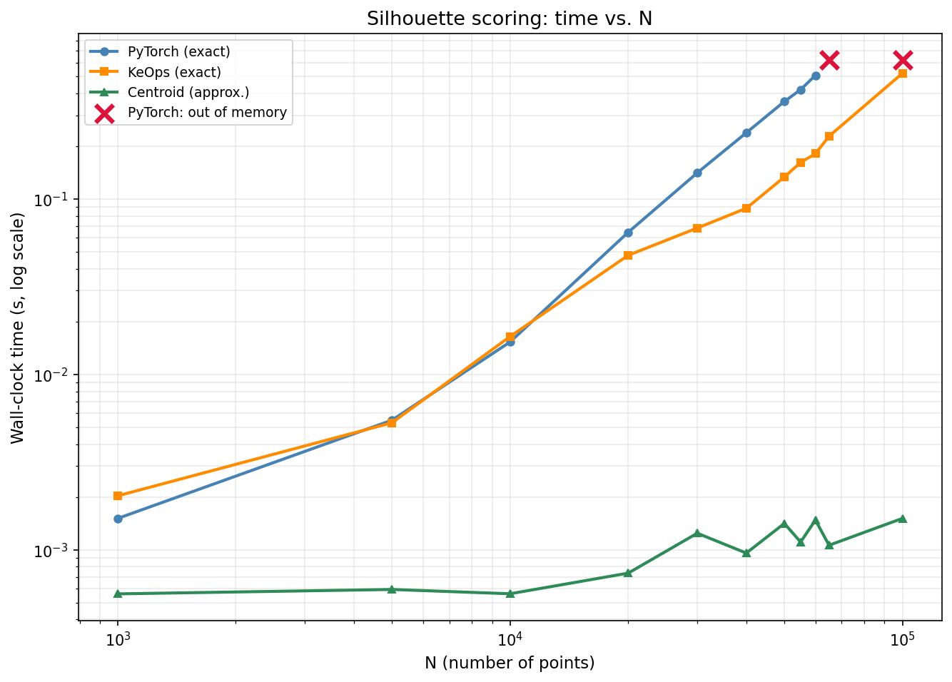
figure 3: time vs. N, log-log, PyTorch / KeOps / Centroid, on a log scale
The more interesting result is the memory behavior. I ran PyTorch, KeOps, and the centroid approximation across a range of N from 1,000 up to 100,000, without any sampling shortcuts, to see how they performed, and if they hit a wall.
PyTorch’s memory grows with the square of N, since exact silhouette scoring needs the full set of pairwise distances, not just distances to a handful of centroids. It held up through 60,000 points at just over 14 GB, finally failing at 65,000 on a 16 GB card. KeOps, computing the identical exact score, never came close to that ceiling. Its memory stayed under 15 MB the entire way, growing linearly rather than the steep curve PyTorch was on (since this is shown on a log scale, below, the Pytorch curve looks like a straight line).
With k-means, KeOps let me scale into the millions of points. Silhouette has a much lower ceiling, topping out in the low hundreds of thousands before memory limits it again. That’s because silhouette scoring needs every pairwise distance, not just distance to K centroids, as k-means does.
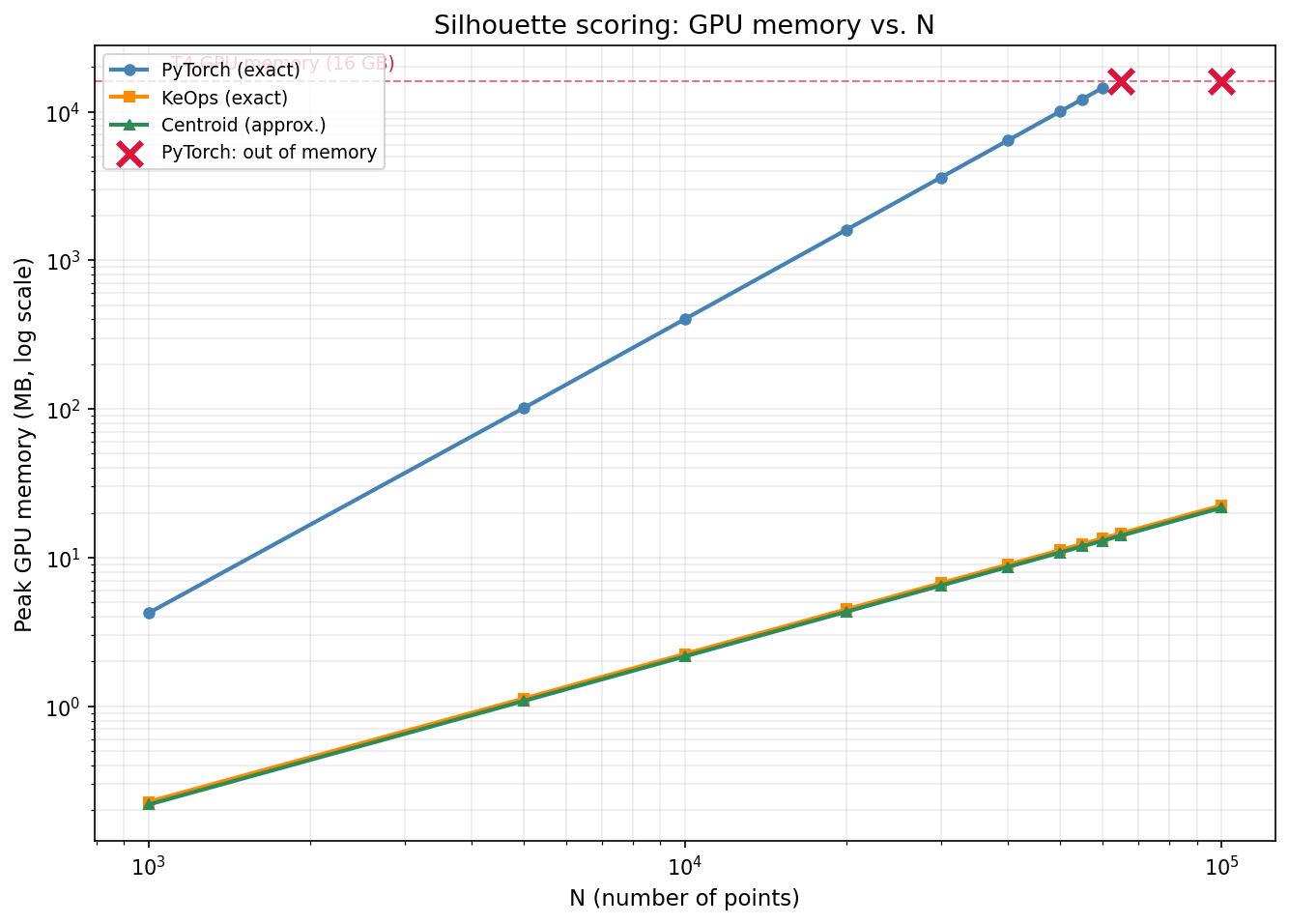
figure 4: memory vs. N, log-log, PyTorch / KeOps / Centroid, OOM marker where PyTorch fails, also on a log scale. Look closely to see the orange KeOps line parallel to the green Centroid line.
For k-means, KeOps improved memory and speed together, since K stays small and fixed. For both the KeOps silhouette implementation, (and the PyTorch implementation), the computation is O(N squared) as every point’s distance to every other point has to be computed. KeOps avoids ever materializing that full matrix in memory, which keeps it from crashing, but it still does the same order of work to produce the result.
The centroid approximation is fast at any scale, since it reduces to the same kind of N times K computation as the k-means assignment step, and it stays under 22 MB even at 100,000 points. If you need silhouette scores at a scale where the exact methods can’t run at all, this is the only real option.
What This Confirmed
This was an extension of the previous work on k-means. Applying a similar framework to a different algorithm family let me verify that the same conclusions generally hold: GPUs can speed up these algorithms, but they may require a KeOps implementation to be practical at scale and avoid memory blowup. For these silhouette tests I found that an approximation algorithm (Centroid) could provide reasonable results quickly and with low memory, but with some caveats.
The framework mattered as much the second time as the first. Having consistent timing and memory measurement, a range of dataset scales, and a verified reference implementation already in place meant I could focus on the silhouette implementations themselves rather than rebuilding infrastructure. Without it I’d have had no reliable way to know if a new implementation was actually correct. I was able to quickly step through a variety of tests with different scales of data to fully understand the performance of the various algorithms.
Simple, non-GPU algorithms have good time and memory performance when working with small datasets such as the Wine set (a few hundred points). It is a general rule of thumb that GPU implementations only pay off once you’re dealing with datasets large enough that algorithm speed becomes an issue. As these tests demonstrate, even larger datasets may start to hit GPU memory limits, requiring something like a KeOps implementation. Truly enormous datasets may not fit into GPU memory at all, even with KeOps, and require sampling or approximations instead.
Next Steps
I realized as I was working on this post that I’ve spent a lot of time on k-means, silhouette scoring, GPU usage, and KeOps, without saying much about the notebook where all of this work actually lives. I’m also not convinced everyone reading these posts is familiar with Jupyter notebooks, what they’re good for, or where they fall short. So the next post, likely the last in this series, steps back from the algorithms and looks at the notebook itself, and at working with notebooks in general.